Examples
This page provides worked examples showing how to use radpair to
simulate cw-EPR spectra of spin-correlated radical pairs. All examples
use types.SimpleNamespace objects to define the spin system,
experiment, and simulation options, which is the simplest way to get
started.
The example scripts are available in the examples/ directory of the
source distribution. Each script is self-contained and can be run with:
uv run python examples/<script_name>.py
Note
The examples require Matplotlib
for plotting, which is included in the dev dependencies. Install with
uv sync --dev or pip install matplotlib.
Common setup
All seven example spectra share the same X-band experiment and simulation options:
from types import SimpleNamespace
import numpy as np

# Experiment: X-band EPR, 9.75 GHz, field sweep 344–350 mT
field_axis = np.linspace(344.0, 350.0, 500)

experiment = SimpleNamespace(
    B_z=field_axis,
    freq_mw=9.75e9,            # Hz
    magnetic_field=field_axis.copy(),
)

# Simulation options: 12 orientation grid knots, single core
simopt = SimpleNamespace(
    grid_points=12,
    refinement=1,
    cpu_cores=1,
)
The do_simulation() function takes three arguments
— spinsystem, experiment, simopt — and returns a
real-valued intensity array matching the shape of experiment.B_z.
from radpair.core import do_simulation

intensity = do_simulation(spinsystem, experiment, simopt)
Unit conventions
Attribute |
Unit |
|---|---|
|
milliTesla |
|
Hz |
|
MHz (3-element arrays) |
|
MHz |
|
MHz |
|
|
|
radians (Euler angles [α, β, γ]) |
|
|
|
number of equivalent nuclei (int ≥ 0) |
|
nuclear spin (float, multiple of ½, ≥ 0) |
Example 1: Bare radical pair (S1)
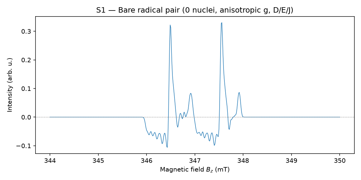
The simplest anisotropic radical pair: two radicals with anisotropic g-tensors, nonzero ZFS (D = 8 MHz, E = 1.5 MHz) and exchange (J = 2 MHz), but no resolved hyperfine couplings.
spinsystem = SimpleNamespace(
    g1=np.array([2.0023, 2.0040, 2.0060]),
    g2=np.array([2.0080, 2.0100, 2.0120]),
    A1=np.array([0.0, 0.0, 0.0]),
    A2=np.array([0.0, 0.0, 0.0]),
    A3=np.array([0.0, 0.0, 0.0]),
    A4=np.array([0.0, 0.0, 0.0]),
    A5=np.array([0.0, 0.0, 0.0]),
    D=8.0, E=1.5, J_ex=2.0,
    width_gauss=0.05,
    g1_frame=np.array([0.1, 0.2, 0.0]),
    g2_frame=np.array([0.0, 0.3, 0.1]),
    D_frame=np.array([0.2, 0.1, 0.0]),
    A1_frame=np.array([0.0, 0.0, 0.0]),
    A2_frame=np.array([0.0, 0.0, 0.0]),
    A3_frame=np.array([0.0, 0.0, 0.0]),
    A4_frame=np.array([0.0, 0.0, 0.0]),
    A5_frame=np.array([0.0, 0.0, 0.0]),
    n1=0, I1=0.0, n2=0, I2=0.0,
    n3=0, I3=0.0, n4=0, I4=0.0, n5=0, I5=0.0,
    donor_list=[], acceptor_list=[],
)

intensity = do_simulation(spinsystem, experiment, simopt)
Example 2: Single donor nucleus, isotropic (S2)
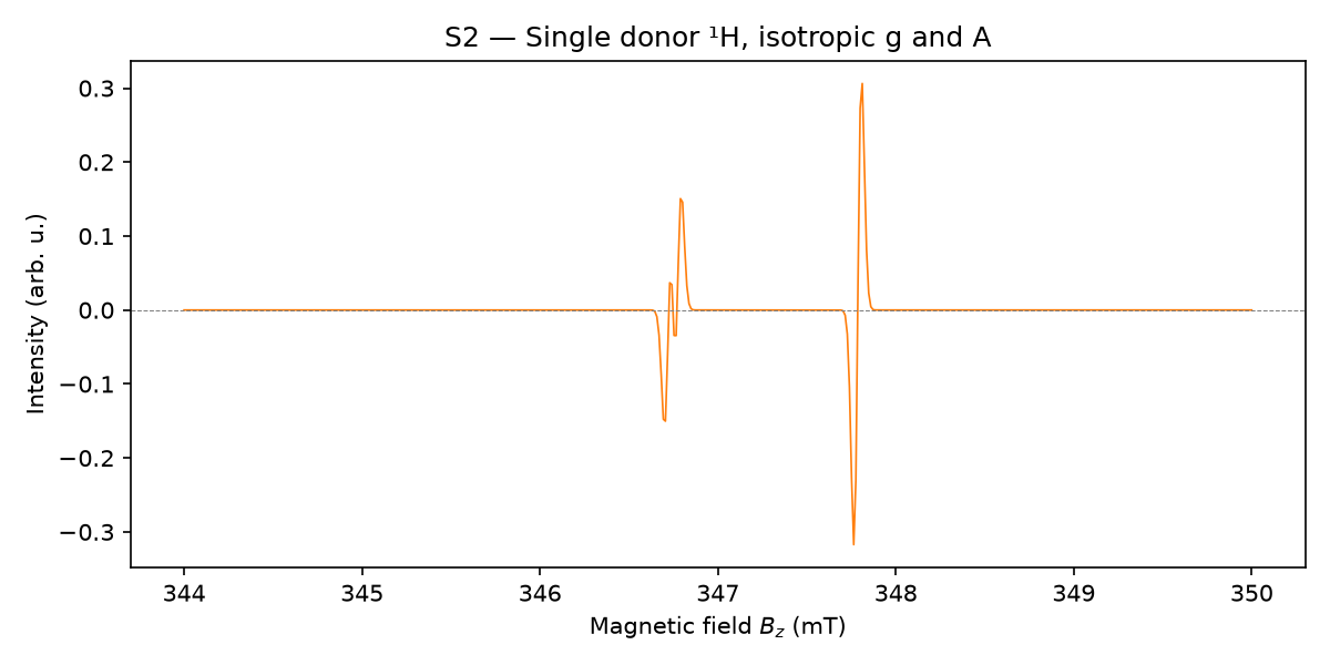
One donor proton with isotropic g-tensors and isotropic hyperfine coupling (A = 1.5 MHz). The acceptor is “silent” (no nuclei, isotropic g). A small exchange (J = 0.1 MHz) is present; ZFS is zero.
spinsystem = SimpleNamespace(
    g1=np.array([2.0030, 2.0030, 2.0030]),
    g2=np.array([2.0090, 2.0090, 2.0090]),
    A1=np.array([1.5, 1.5, 1.5]),
    A2=np.array([0.0, 0.0, 0.0]),
    A3=np.array([0.0, 0.0, 0.0]),
    A4=np.array([0.0, 0.0, 0.0]),
    A5=np.array([0.0, 0.0, 0.0]),
    D=0.0, E=0.0, J_ex=0.1,
    width_gauss=0.05,
    g1_frame=np.array([0.0, 0.0, 0.0]),
    g2_frame=np.array([0.0, 0.0, 0.0]),
    D_frame=np.array([0.0, 0.0, 0.0]),
    A1_frame=np.array([0.0, 0.0, 0.0]),
    A2_frame=np.array([0.0, 0.0, 0.0]),
    A3_frame=np.array([0.0, 0.0, 0.0]),
    A4_frame=np.array([0.0, 0.0, 0.0]),
    A5_frame=np.array([0.0, 0.0, 0.0]),
    n1=1, I1=0.5, n2=0, I2=0.0,
    n3=0, I3=0.0, n4=0, I4=0.0, n5=0, I5=0.0,
    donor_list=[1], acceptor_list=[],
)
Example 3: Two anisotropic nuclei, mixed donor/acceptor (S3)
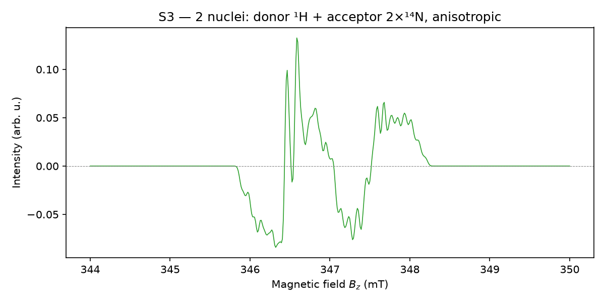
A more realistic system: the donor carries one ¹H with anisotropic hyperfine coupling (A*₁ = [5, 3, 4] MHz), and the acceptor carries two equivalent ¹⁴N nuclei (*I = 1, n = 2, A*₂ = [2.5, 1.8, 3.2] MHz). Both g-tensors are anisotropic, and ZFS (*D = 8, E = 1.5 MHz) and exchange (J = 3 MHz) are nonzero. Several Euler frames are nonzero, so tensors are rotated relative to the lab frame.
spinsystem = SimpleNamespace(
    g1=np.array([2.0020, 2.0040, 2.0060]),
    g2=np.array([2.0080, 2.0100, 2.0120]),
    A1=np.array([5.0, 3.0, 4.0]),
    A2=np.array([2.5, 1.8, 3.2]),
    A3=np.array([0.0, 0.0, 0.0]),
    A4=np.array([0.0, 0.0, 0.0]),
    A5=np.array([0.0, 0.0, 0.0]),
    D=8.0, E=1.5, J_ex=3.0,
    width_gauss=0.05,
    g1_frame=np.array([0.1, 0.2, 0.0]),
    g2_frame=np.array([0.0, 0.3, 0.1]),
    D_frame=np.array([0.2, 0.1, 0.0]),
    A1_frame=np.array([0.0, 0.1, 0.0]),
    A2_frame=np.array([0.1, 0.0, 0.0]),
    A3_frame=np.array([0.0, 0.0, 0.0]),
    A4_frame=np.array([0.0, 0.0, 0.0]),
    A5_frame=np.array([0.0, 0.0, 0.0]),
    n1=1, I1=0.5, n2=2, I2=1.0,
    n3=0, I3=0.0, n4=0, I4=0.0, n5=0, I5=0.0,
    donor_list=[1], acceptor_list=[2],
)
Example 4: Donor/acceptor swap (S3 vs S4)
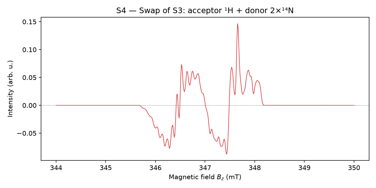
Systems S3 and S4 are identical except that the donor and acceptor nuclei assignments are swapped. This demonstrates how the same nuclei produce different spectra depending on which radical they belong to — the MHz-to-Tesla conversion uses different g-tensors for donor vs. acceptor nuclei.
# S4: same as S3 but with swapped assignments
spinsystem_S4 = SimpleNamespace(
    # ... (same g, A, D, E, J_ex, frames as S3) ...
    donor_list=[2],      # was [1] in S3
    acceptor_list=[1],   # was [2] in S3
)

intensity_S3 = do_simulation(spinsystem_S3, experiment, simopt)
intensity_S4 = do_simulation(spinsystem_S4, experiment, simopt)
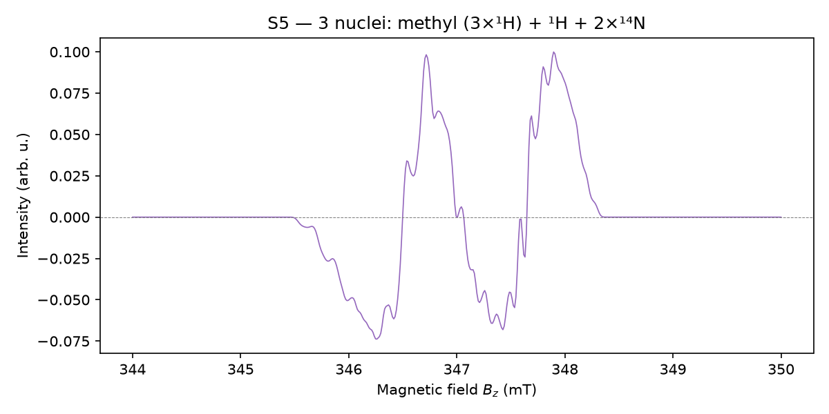
Example 5: Three nuclei with methyl group (S5)
Donor with a methyl group (3 equivalent ¹H, n = 3) plus a single ¹H, acceptor with 2 equivalent ¹⁴N. All tensors are anisotropic.
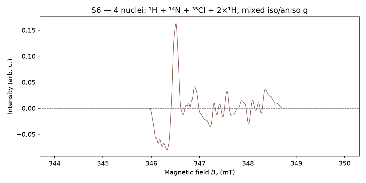
Example 6: Four nuclei with ³⁵Cl (S6)
Donor with one ¹H, acceptor with ¹⁴N + ³⁵Cl (I = 3/2) + 2×¹H. The donor g-tensor is isotropic while the acceptor g-tensor is anisotropic.
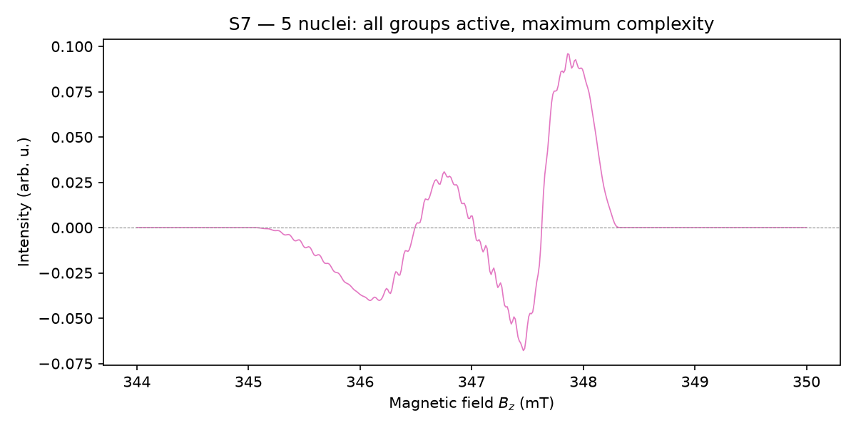
Example 7: Five nuclei, maximum complexity (S7)
All five nuclei groups are active (3 donor + 2 acceptor), with anisotropic g-tensors, full ZFS (D = 10, E = 2 MHz), exchange (J = 5 MHz), and multiple nuclear spins (I = ½, 1, 3/2) and multiplicities (n = 1, 2).
spinsystem = SimpleNamespace(
    g1=np.array([2.0020, 2.0040, 2.0060]),
    g2=np.array([2.0080, 2.0100, 2.0120]),
    A1=np.array([4.5, 3.0, 5.5]),
    A2=np.array([2.0, 1.5, 2.8]),
    A3=np.array([6.0, 4.0, 8.0]),
    A4=np.array([1.5, 1.0, 2.0]),
    A5=np.array([3.0, 2.0, 4.0]),
    D=10.0, E=2.0, J_ex=5.0,
    width_gauss=0.05,
    g1_frame=np.array([0.1, 0.2, 0.0]),
    g2_frame=np.array([0.0, 0.3, 0.1]),
    D_frame=np.array([0.2, 0.1, 0.0]),
    A1_frame=np.array([0.1, 0.0, 0.0]),
    A2_frame=np.array([0.0, 0.1, 0.0]),
    A3_frame=np.array([0.1, 0.1, 0.0]),
    A4_frame=np.array([0.0, 0.0, 0.0]),
    A5_frame=np.array([0.0, 0.0, 0.0]),
    n1=1, I1=0.5, n2=2, I2=1.0, n3=1, I3=1.5,
    n4=1, I4=0.5, n5=2, I5=0.5,
    donor_list=[1, 2, 3], acceptor_list=[4, 5],
)
Multi-core simulation
For computationally expensive systems, do_simulation_multicore()
splits the field axis across multiple CPU processes via
multiprocessing.Pool. The result is numerically identical to
the single-core call.
from radpair.core import do_simulation_multicore

simopt_multicore = SimpleNamespace(
    grid_points=12,
    refinement=1,
    cpu_cores=4,   # use 4 worker processes (0 = auto-detect)
)

intensity = do_simulation_multicore(spinsystem, experiment, simopt_multicore)
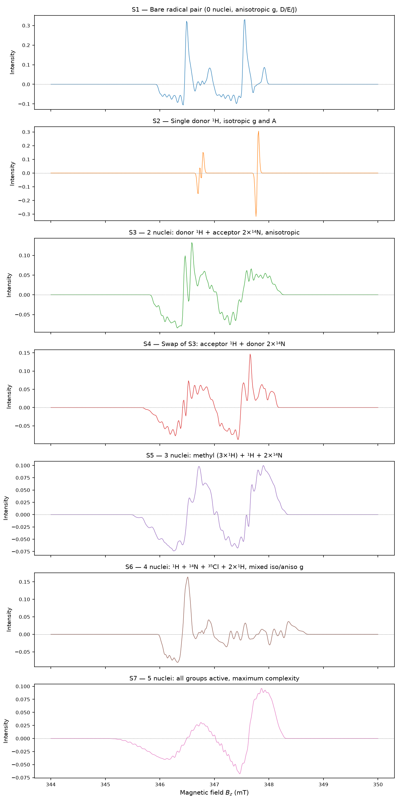
Overview of all seven example spectra (S1–S7), showing the increasing spectral complexity as more nuclei groups are added.
Available example scripts
All scripts are in the examples/ directory and can be run individually:
Script |
Description |
|---|---|
|
S1: bare radical pair, 0 nuclei |
|
S2: single donor ¹H, isotropic |
|
S3: 2 nuclei, mixed donor/acceptor, anisotropic |
|
S3 vs S4: donor/acceptor swap comparison |
|
S7: 5 nuclei, maximum complexity |
|
Multi-core simulation demo |
|
Generate all 7 spectra plots for the docs |